tidymst reads microscale thermophoresis (MST) data from NanoTemper’s software into tidy data frames, and analyses them:
- Read MST traces, capillary scans, dose-response data and fits with
read_mst()and friends, from either the Excel files exported by MO.Affinity Analysis or the project files saved by MO.Control (.moc) and MO.Affinity Analysis (.nta). Everything is read into the same standard columns, with concentrations in molar. - Recalculate Fnorm from the traces with any hot and cold windows, using
mst_fnorm(). - Fit Kd and Hill binding models with
mst_fit(), and get the coefficients and curves withmst_coefs()andmst_curve(). - Convert responses to delta Fnorm and fraction bound with
mst_normalise(). - Plot traces and dose-response curves with
mst_plot_traces()andmst_plot_dose_response(), or with your own ggplot2 code.
Installation
Install the development version of tidymst from GitHub with:
# install.packages("pak")
pak::pak("BradyAJohnston/tidymst")
Example
Read the MST traces exported from MO.Affinity Analysis, calculate Fnorm for the capillaries that weren’t marked as outliers, and fit a Kd:
library(tidymst)
library(dplyr)

traces <- read_mst_traces(tidymst_example("dppr10-cy5_traces.xlsx"))

fnorm <- traces |>
  filter(included, target == "atpH-fl") |>
  mst_fnorm(hot = c(19, 20))

fits <- mst_fit(fnorm, .by = target)
mst_coefs(fits)
#> # A tibble: 4 × 7
#>   target  model term                 estimate     std_error conf_low conf_high
#>   <chr>   <chr> <chr>                   <dbl>         <dbl>    <dbl>     <dbl>
#> 1 atpH-fl kd    unbound               1.09e+3 1.74           1.09e+3   1.10e+3
#> 2 atpH-fl kd    bound                 8.52e+2 2.80           8.46e+2   8.58e+2
#> 3 atpH-fl kd    kd                    1.26e-8 0.00000000367  6.99e-9   2.27e-8
#> 4 atpH-fl kd    target_concentration  1.20e-7 0.00000000951  1.02e-7   1.40e-7
mst_plot_dose_response(fnorm, fits)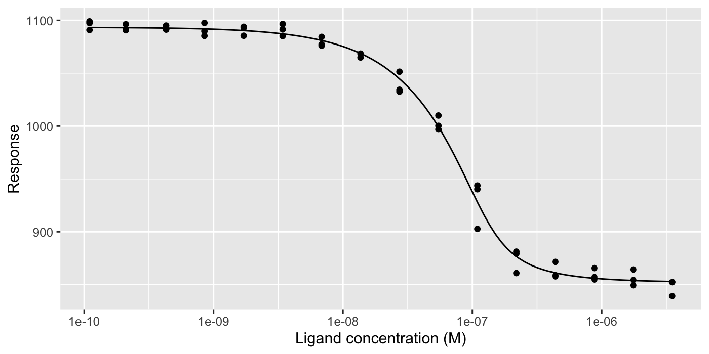
Reading project files
You don’t need to export anything: the same functions read the project files that NanoTemper’s software saves. An MO.Affinity Analysis project (.nta) holds the raw measurements and your analysis, including which capillaries are outliers and the fits:
project <- tidymst_example("dppr10-cy5.nta")

read_mst_dose_response(project) |>
  select(target, ligand_concentration, response, included)
#> # A tibble: 80 × 4
#>    target  ligand_concentration response included
#>    <chr>                  <dbl>    <dbl> <lgl>
#>  1 atpH-fl        0.0000035         839. TRUE
#>  2 atpH-fl        0.00000175        849. TRUE
#>  3 atpH-fl        0.000000875       855. TRUE
#>  4 atpH-fl        0.000000438       858. TRUE
#>  5 atpH-fl        0.000000219       861. TRUE
#>  6 atpH-fl        0.000000109       903. TRUE
#>  7 atpH-fl        0.0000000547      997. TRUE
#>  8 atpH-fl        0.0000000273     1034. TRUE
#>  9 atpH-fl        0.0000000137     1065. TRUE
#> 10 atpH-fl        0.00000000684    1076. TRUE
#> # ℹ 70 more rows

read_mst_fit(project) |>
  select(target, model, fixed, kd, kd_std_error)
#> # A tibble: 3 × 5
#>   target   model fixed            kd kd_std_error
#>   <chr>    <chr> <chr>         <dbl>        <dbl>
#> 1 atpH-fl  hill  <NA>  NA                NA
#> 2 atpH-fl  kd    bound  0.0000000144      2.04e-9
#> 3 NEAT1-fl kd    <NA>   0.000000434      NA
An MO.Control project (.moc) holds the measurements only, so it gives traces and capillary scans.
See vignette("tidymst") for a full walk-through, including how to make your own plots.