A complete MDAnalysis workflow on the AdK equilibrium dataset, rendering with Molecular Nodes along the way.
This page walks through a full analysis of a molecular dynamics trajectory with MDAnalysis, using Molecular Nodes for the pictures along the way and a rendered animation at the end. It follows the same workflow as the MDAnalysis User Guide examples for RMSD and RMSF and native contacts and the domain-angle analysis from the classic MDAnalysis tutorial. Those examples visualise their results with the browser-based nglview; here every render is produced by Blender through the Molecular Nodes Python API instead, so the same code that makes a quick preview in a notebook also makes a publication figure or a movie.
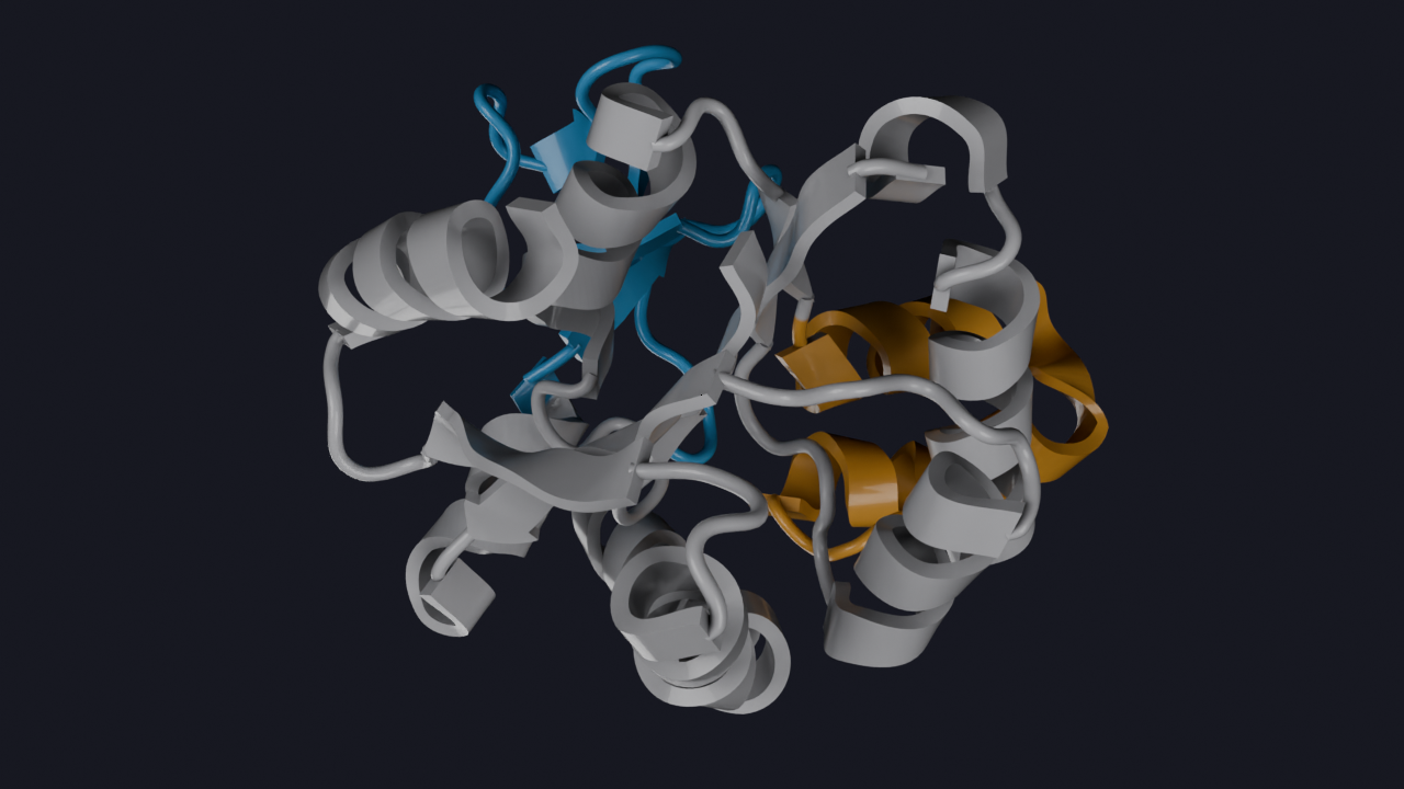
The system is adenylate kinase (AdK), a 214-residue enzyme with three domains that open and close around the active site: the rigid CORE, the NMP binding domain (residues 30-59) and the LID domain (residues 122-159). The AdK equilibrium dataset from MDAnalysisData is a 1 µs simulation of the apo protein, saved every 240 ps (4187 frames) with the solvent stripped, so it is small enough (161 MB) to download during a workshop.
Molecular Nodes runs on the bpy module, which is Blender as a regular Python package. Blender pins the Python version tightly, so the environment must be Python 3.13. The easiest way to get a working environment is with uv, which creates and manages the virtual environment for you:
molecularnodes[bpy] installs Blender itself (bpy, around 300 MB) alongside Molecular Nodes and its dependencies, which already include MDAnalysis.
[jupyter] adds Jupyter and Pillow, so rendered images and videos display inline in a notebook. Molecular Nodes works from a plain script too, in which case pass path= to the render calls to save files instead.
MDAnalysisData provides the example datasets. The first call to a fetch_* function downloads the data into ~/MDAnalysis_data/ and later calls reuse the cached copy.
Start a notebook with uv run jupyter lab (or jupyter lab in the activated environment) and check that everything imports:
import molecularnodes as mnfrom molecularnodes.nodes import geometry as mgfrom nodebpy import geometry as gfrom nodebpy import shader as simport MDAnalysis as mdafrom MDAnalysis.analysis import align, rmsfrom MDAnalysisData import datasetsimport numpy as npimport pandas as pdimport matplotlib.pyplot as pltprint(f"MDAnalysis {mda.__version__}")
MDAnalysis 2.10.0
TipRendering without a GPU
Everything on this page renders on the CPU. If your machine has no GPU (a laptop, a cloud notebook or a cluster node), also switch the compositor to the CPU right after creating the canvas: canvas.compositor.device = "CPU". Blender defaults it to the GPU and aborts the render on a machine without one.
Create the canvas
The Canvas is the handle on the Blender scene: render engine, resolution, camera and lighting all live here. Create it before loading any structures. Still images use Cycles with a modest sample count, which takes around ten seconds per frame on a laptop CPU.
MDAnalysisData returns a bunch with the paths to the topology and trajectory files, plus a DESCR string describing the simulation. Everything else is standard MDAnalysis: a Universe that we will analyse and render.
<Universe with 3341 atoms>
4187 frames, 240 ps apart, 1.00 µs in total
The three domains are defined by residue ranges. We keep the MDAnalysis selection strings in one dictionary, and a colour for each, so the analysis and the renders always agree on what a domain is.
A Molecule wraps the Universe and creates the object in the Blender scene. It stays linked to the Universe: changing the scene frame steps the trajectory, and transformations applied in MDAnalysis show up in the render.
traj = mn.Molecule(u)
A custom material
Rather than one of the pre-built materials, we build one from scratch with nodebpy’s shader nodes. The MNColor node reads the per-atom colours that the geometry nodes produce, some ambient occlusion darkens the crevices, and a coat on the Principled BSDF gives the cartoon a glossy finish. fake_user=True keeps the material alive when the scene is cleared later on, so the animation at the end can reuse it.
with s.material("Glossy Domains", fake_user=True) as glossy:
    glossy.nodes.clear()
    color = mn.nodes.shader.MNColor()
    ao = s.AmbientOcclusion(color, distance=0.4, samples=32)
    bsdf = s.PrincipledBSDF(base_color=ao.o.color, roughness=0.3, coat_weight=0.5)
    bsdf >> s.MaterialOutput().i.surface
Styling with the node tree
add_style covers the common cases, but for anything with several steps we build the geometry node tree directly with mol.tree. Inside the with block, >> links one node into the next, atoms is the raw atomic data coming in and join collects everything that should be rendered.
Each domain gets a Set Color node whose selection is an MDAnalysis selection string turned into a node with node. The PSF topology carries no secondary structure, so a Topology DSSP node computes it per frame before the cartoon is built.
def color_domains(mol, atoms):"""Chain one Set Color node per domain onto `atoms` and return the result."""for name, selection in DOMAINS.items(): atoms = atoms >> mg.SetColor( selection=mol.selections.node(selection), color=DOMAIN_COLORS[name], )return atomswith traj.tree.reset() as (atoms, join): ( color_domains(traj, atoms)>> mg.TopologyDSSP()>> mg.StyleCartoon(quality=4, material=glossy.material)>> join )canvas.look_at(traj, viewpoint="top", margin=0.15)canvas.snapshot()
Figure 1: AdK coloured by domain — CORE in grey, NMP in orange and LID in blue — with the custom glossy material.
Note
The order of the nodes matters: anything placed between the Topology DSSP node and the style node — a Set Color, a transform — is not picked up by the style. Put every colour and transform node first and compute the secondary structure immediately before the style node.
RMSD of each domain
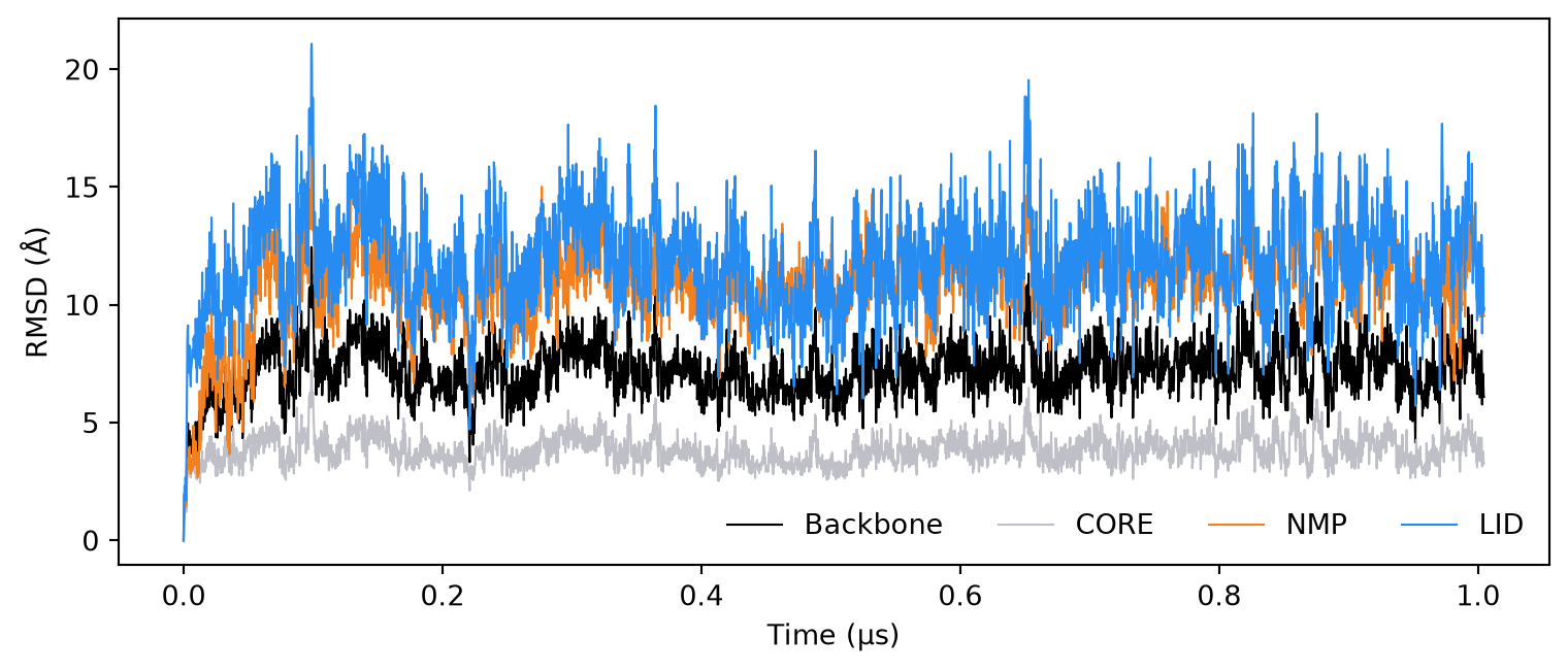
The root-mean-square deviation from the first frame shows how far the protein drifts over the simulation. Passing groupselections computes the RMSD of each domain in the same pass, after superimposing on the backbone, exactly as in the User Guide’s RMSD example.
R = rms.RMSD( u, u, select="backbone", groupselections=[f"backbone and ({sel})"for sel in DOMAINS.values()], ref_frame=0,).run()rmsd = pd.DataFrame( R.results.rmsd, columns=["Frame", "Time (ps)", "Backbone", *DOMAINS],)rmsd.head()
Figure 2: Backbone RMSD to the first frame for the whole protein and for each domain.
The CORE barely moves while the LID and NMP domains swing by several ångströms: the motion we are looking at is the domains moving relative to a stable core.
Per-residue flexibility (RMSF)
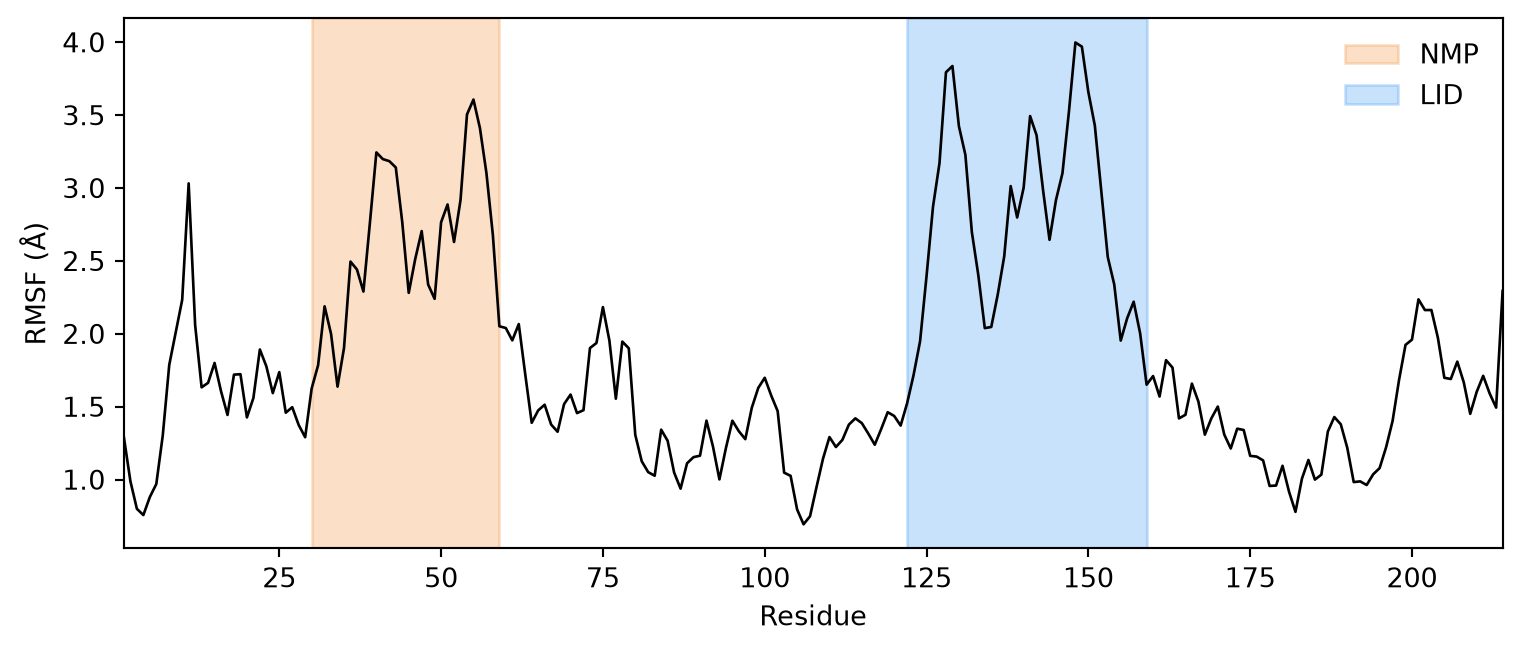
The root-mean-square fluctuation tells us where the protein is flexible. Following the User Guide’s RMSF example, we first align every frame onto the average structure of the α-carbons. The alignment is done in memory, so from here on the Universe (and therefore our Molecule) holds the aligned coordinates.
average = align.AverageStructure(u, u, select="protein and name CA", ref_frame=0).run()reference = average.results.universealign.AlignTraj(u, reference, select="protein and name CA", in_memory=True).run()c_alphas = u.select_atoms("protein and name CA")rmsf = rms.RMSF(c_alphas).run()
Figure 3: RMSF of the α-carbons. The shaded regions mark the NMP and LID domains.
Colouring the render by a computed value
Any per-atom array can be stored on the Molecule as a named attribute, where the node tree can read it. The RMSF is one value per residue, so we broadcast it to every atom of that residue through resindices before storing it.
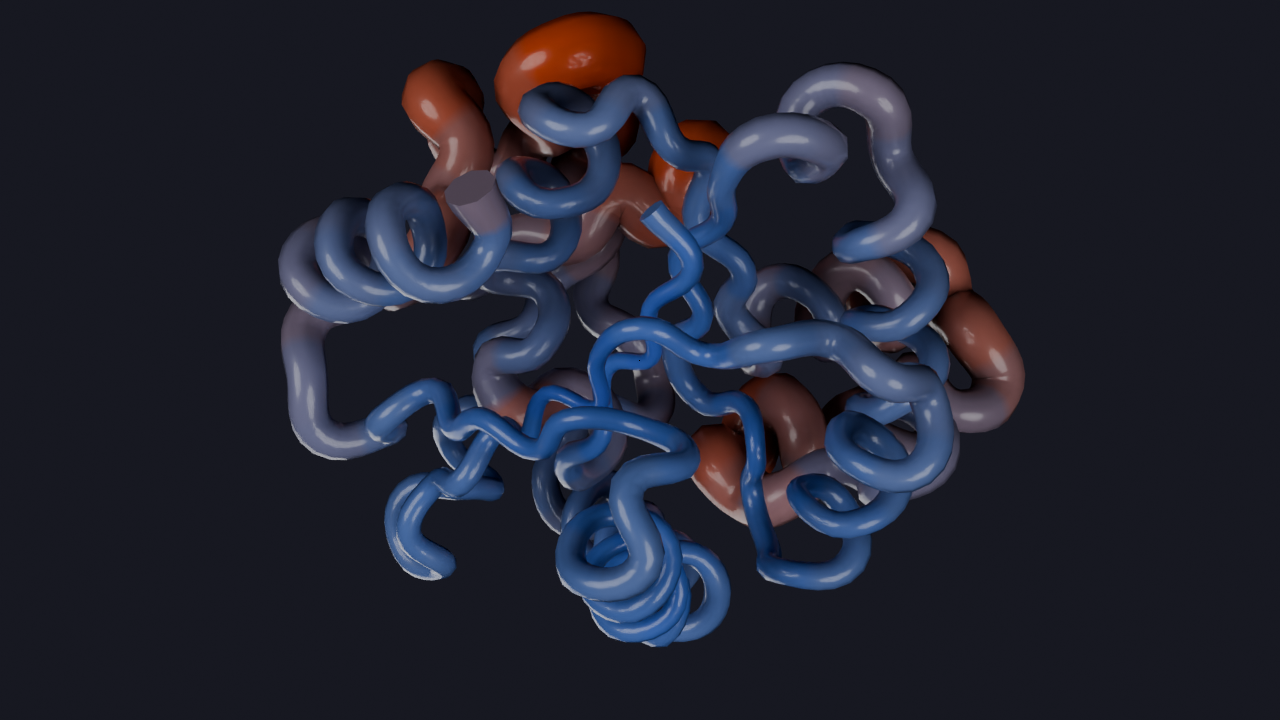
The Color Attribute Map node turns the stored value into a colour between two end-points, and the same attribute drives the size of a sphere on each α-carbon through a Map Range node. Because both styles are branches of the same node tree, they share the coloured atoms and are joined back together for rendering.
Figure 4: Cartoon coloured by RMSF, from blue (rigid) to red (flexible). The spheres on the α-carbons are scaled by the same value.
Domain opening and closing
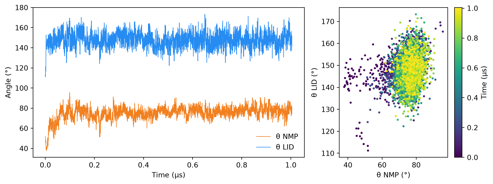
The functional motion of AdK is the LID and NMP domains closing over the active site. It is usually described by two angles between centres of geometry of groups of residues, following Beckstein et al. (2009): θNMP between the NMP domain and the CORE, and θLID between the LID domain and the CORE.
def backbone(resids):return u.select_atoms(f"resid {resids} and (backbone or name CB)")def angle(a, b, c):"""Angle in degrees at `b` between the centres of geometry of three groups.""" ba = a.center_of_geometry() - b.center_of_geometry() bc = c.center_of_geometry() - b.center_of_geometry() cosine = np.dot(ba, bc) / (np.linalg.norm(ba) * np.linalg.norm(bc))return np.degrees(np.arccos(cosine))nmp_groups = (backbone("35:55"), backbone("90:100"), backbone("115:125"))lid_groups = (backbone("125:153"), backbone("115:125"), backbone("179:185"))angles = pd.DataFrame( [(ts.time /1e6, angle(*nmp_groups), angle(*lid_groups)) for ts in u.trajectory], columns=["Time (µs)", "NMP", "LID"],)angles.describe().loc[["min", "mean", "max"]]
Figure 5: The two domain angles over time (left) and against each other (right), coloured by simulation time.
Rendering the extremes
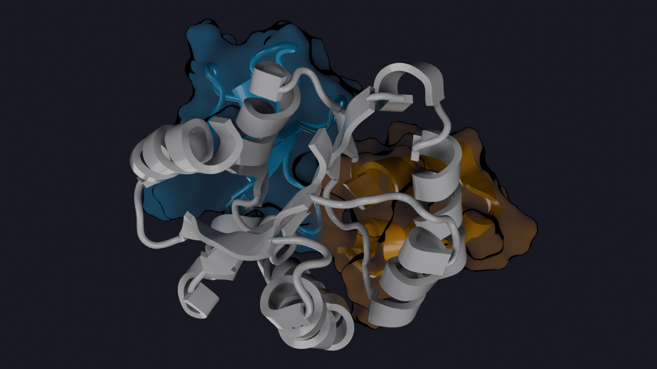
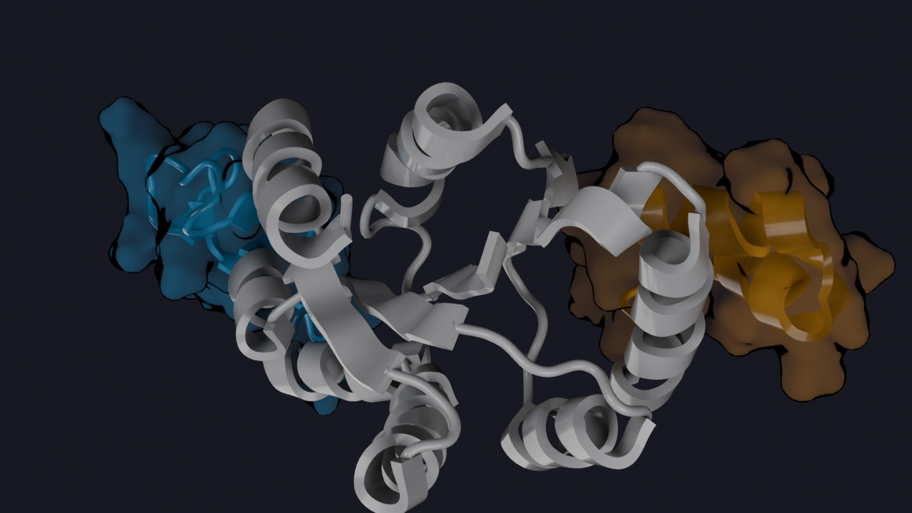
The angles let us pick specific frames to look at: the most closed conformation (smallest angles) and the most open one. The Molecule follows the scene frame, so snapshot with frame= renders any frame of the trajectory without touching the Universe ourselves.
For the render we add a second branch to the tree: a transparent surface over just the two mobile domains, using the pre-built Transparent material with a Fresnel rim so the surface reads as a volume without hiding the cartoon underneath.
rim = mn.material.Transparent(transparency=0.75, fresnel=True)mobile =f"{DOMAINS['NMP']} or {DOMAINS['LID']}"with traj.tree.reset() as (atoms, join): colored = color_domains(traj, atoms) >> mg.TopologyDSSP() colored >> mg.StyleCartoon(quality=4, material=glossy.material) >> join ( colored>> mg.StyleSurface( selection=traj.selections.node(mobile), quality=3, material=rim.material, )>> join )canvas.look_at(traj, viewpoint="top", margin=0.1)for frame in (closed_frame, open_frame): display(canvas.snapshot(frame=frame))
(a) Closed
(b) Open
Figure 6: The most closed and most open conformations sampled in the simulation, with a transparent surface over the LID and NMP domains.
The contacts that hold the domains together
The simulation starts from the closed crystal structure and opens within the first few nanoseconds, so the interesting part of the trajectory for a movie is the very beginning. Before rendering it, we find what actually ties the LID and NMP domains together in that closed starting frame. A capped distance search between the heavy atoms of the two domains returns every pair within 4.5 Å, and from the pairs we read off the residues involved.
from MDAnalysis.analysis import contactsfrom MDAnalysis.lib import distanceslid_heavy = u.select_atoms(f"({DOMAINS['LID']}) and not name H*")nmp_heavy = u.select_atoms(f"({DOMAINS['NMP']}) and not name H*")u.trajectory[0]pairs, _ = distances.capped_distance( lid_heavy.positions, nmp_heavy.positions, max_cutoff=4.5)contact_lid = lid_heavy[np.unique(pairs[:, 0])].residuescontact_nmp = nmp_heavy[np.unique(pairs[:, 1])].residuesresidue_pairs = { (f"{a.resname}{a.resid}", f"{b.resname}{b.resid}")for a, b inzip(lid_heavy[pairs[:, 0]], nmp_heavy[pairs[:, 1]])}for lid_res, nmp_res insorted(residue_pairs):print(f"LID {lid_res} <-> NMP {nmp_res}")
LID ARG156  <->  NMP ARG36
LID LYS157  <->  NMP ASP54
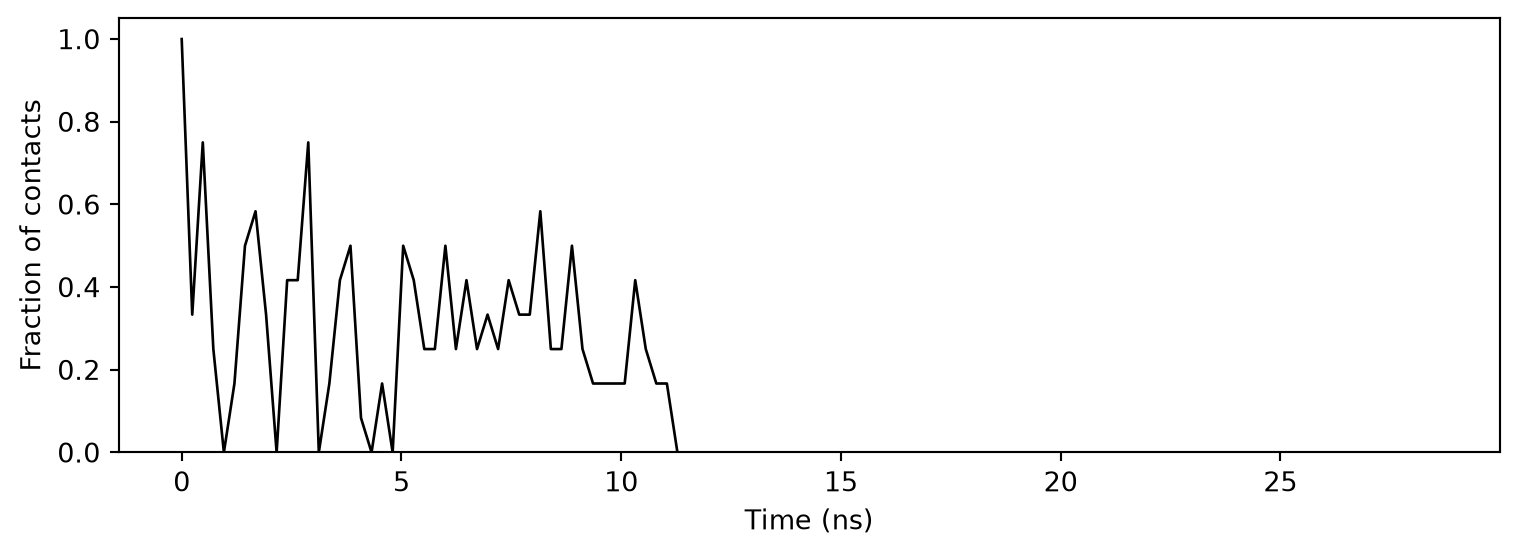
A salt bridge between Lys157 on the LID and Asp54 on the NMP domain, flanked by two arginines, is the only direct contact between the two domains. Following the User Guide’s native contacts example, Contacts tracks the fraction of these starting contacts that survive in every later frame.
Figure 7: Fraction of the initial LID–NMP contacts that remain, over the first 15 ns. The interface is gone within a few nanoseconds and never re-forms for long.
The residues go into one more selection string so that the animation can draw them.
contact_resids = np.concatenate([contact_lid.resids, contact_nmp.resids])CONTACTS ="resid "+" ".join(str(r) for r in contact_resids) +" and not name H*"CONTACTS
'resid 156 157 36 54 and not name H*'
An animation of the salt bridge breaking
The movie covers those first 60 frames (14 ns). The frames are 240 ps apart, which is far too coarse to watch a side chain swing away, so we lean on the playback controls of the Molecule (see Trajectories):
subframes inserts extra scene frames between trajectory frames, and interpolate fills them by interpolating the positions, so four subframes stretch each trajectory frame over five scene frames.
average averages a window of neighbouring frames, which takes the thermal jitter out of the motion so the slower domain opening reads clearly.
clear removes the molecules from the scene while keeping the camera, lights and render settings, and the aligned Universe is wrapped in a fresh Molecule. The animation renders with EEVEE, which is many times faster than Cycles and looks close enough for a movie.
canvas.clear()canvas.engine = mn.scene.EEVEE()canvas.fps =24canvas.resolution = (800, 600)movie = mn.Molecule(u)movie.dssp.init() # compute secondary structure for the moviemovie.subframes =1movie.interpolate =Truemovie.average =1canvas.frame_range = (0, MOVIE_FRAMES * (movie.subframes +1) -1)print(f"{canvas.frame_range[1] +1} scene frames, "f"{(canvas.frame_range[1] +1) / canvas.fps:.1f} s at {canvas.fps} fps")
Info: Deleted 3 data-block(s)
240 scene frames, 10.0 s at 24 fps
The node tree is built once, but Blender re-evaluates it on every frame. A Scene Time node exposes the current frame, and a Map Range turns it into a slow half turn over the length of the animation. After centring the atoms on the CORE domain, a Transform Geometry node applies that rotation, so the protein turns while the trajectory plays underneath it. The transformed atoms then feed two branches: the domain-coloured cartoon (secondary structure computed last, right before the style, as before), and the contact residues drawn as ball-and-stick in a highlight colour so they stand out as the salt bridge is pulled apart.
animation renders the scene’s frame range and returns the video for display. Pass path="adk.mp4" to save it to disk as well. The camera is framed once, with extra margin so the turning protein stays in shot.
(a) The first 14 ns of the simulation, smoothed and interpolated, with the Lys157–Asp54 salt bridge and its neighbouring arginines drawn in yellow as the LID and NMP domains pull apart.
(b)
Figure 8
Where to go next
Swap the dataset: datasets.fetch_adk_transitions_DIMS() holds 200 short trajectories of AdK closing, which make a clean open-to-closed movie, and datasets.fetch_membrane_peptide() is a small peptide in a lipid bilayer.
Compute something else and store it as an attribute — a distance, a hydrogen bond count, a PCA projection — and colour or scale the style by it as we did with the RMSF.
The Styles, Materials and Node Trees pages cover the full set of styles, colour nodes and materials used above, and Rendering covers frame-by-frame recording for animations where the camera or the style should change between frames.