Solvent Density

An example for visualizing solvent density.

This example follows the Calculating the solvent density around a protein example from the MDAnalysis user guide.

import MDAnalysis as mda
import molecularnodes as mn
from MDAnalysis import transformations as trans
from MDAnalysis.analysis import density
from MDAnalysis.tests.datafiles import TPR, XTC

canvas = mn.Canvas()

Load and transform Universe

u = mda.Universe(TPR, XTC)

protein = u.select_atoms("protein")
water = u.select_atoms("not protein")

workflow = [
    trans.unwrap(u.atoms),  # unwrap all fragments
    trans.center_in_box(
        protein,
        center="geometry",  # move atoms to center protein
    ),
    trans.wrap(
        water,
        compound="residues",  # wrap each water back into box
    ),
    trans.fit_rot_trans(
        protein,
        protein,
        weights="mass",  # align protein to first frame
    ),
]

u.trajectory.add_transformations(*workflow)

Analyse and Export `.dx`

ow = u.select_atoms("name OW")
dens = density.DensityAnalysis(ow, delta=4.0, padding=2)
dens.run()
# convert density unit to TIP4P
dens.results.density.convert_density("TIP4P")
dens.results.density.export("water.dx")

Add Universe to Blender

Import universe as a Molecule and add a ribbon style to represent the protein. We also add a style to the non-protein atoms, sliced along the y axis. After taking the snapshot for visual reference we rebuild the tree with just the ribbon style, as we will be showing the water as a density.

from molecularnodes.nodes import geometry as mg
from nodebpy.nodes import geometry as g

t = mn.Molecule(u)

with t.tree.reset() as (atoms, join):
    (
        atoms
        >> mg.StyleRibbon(quality=5, peptide_radius=2)
        >> mg.StyleSpheres(
            selection=g.Position().o.position.y < mg.Centroid(),
            sphere="Instance"
            )
        >> g.SetMaterial(material=mn.material.Default().material)
        >> join
    )
    atoms >> mn.nodes.geometry.StyleRibbon(quality=5, peptide_radius=2) >> join

canvas.look_at(t, (90, 0, 60))
canvas.snapshot()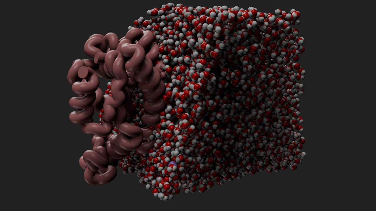

Add density component

We can load the density that was written-out from the analysis performed previously as a Density entity.

# load density file
canvas.engine = "EEVEE"
d = mn.entities.density.Grids.load(
    file_path="water.dx",
    overwrite=True,
)

with d.tree.reset() as (geo, join):
    (
        geo
        >> mg.DensityStyleISOSurface()
        >> g.SetMaterial(material=mn.material.TransparentOutline().material)
        >> join
    )


da = d.annotations.add_density_info()
da.show_origin = da.show_delta = da.show_shape = False

Visualization

Set density style values

# get the density style
# ds = d.styles[0]
# set the positive color to blue with 50% opacity
# ds.positive_color = (0, 0, 1, 0.5)

ISO Value 0.5

# set ISO value to 0.5
# ds.iso_value = 0.5

# frame the density component and render
canvas.look_at(d, viewpoint="front")
canvas.snapshot()

ISO Value 0.5 with Contours

# set ISO value to 0.5
# ds.iso_value = 0.5
# # enable contours
# ds.show_contours = True
# # set contour thickness
# ds.contour_thickness = 0.25
# # set contour colors
# ds.contour_color = (1, 1, 1, 1)

# frame the density component and render
canvas.look_at(d.get_view(), viewpoint="front")
canvas.snapshot()

From Top with Grid Axes

# add grid axes annotation
ga = d.annotations.add_grid_axes_3d()

# set viewpoint to top
canvas.look_at(d.get_view(), viewpoint="top")
display(canvas.snapshot())
# hide grid axes
ga.visible = False

ISO Value 0.5 sliced from Left

# slice the grid from the left 50%
# ds.slice_left = 50

# set viewpoint to left
canvas.look_at(d.get_view(), viewpoint="left")
canvas.snapshot()

Only Contours

# reset slicing
# ds.slice_left = 0
# # only show contours
# ds.only_contours = True

# set viewpoint to front
canvas.look_at(d.get_view(), viewpoint="front")
canvas.snapshot()